Polynomial Regression for Digital Ads with R

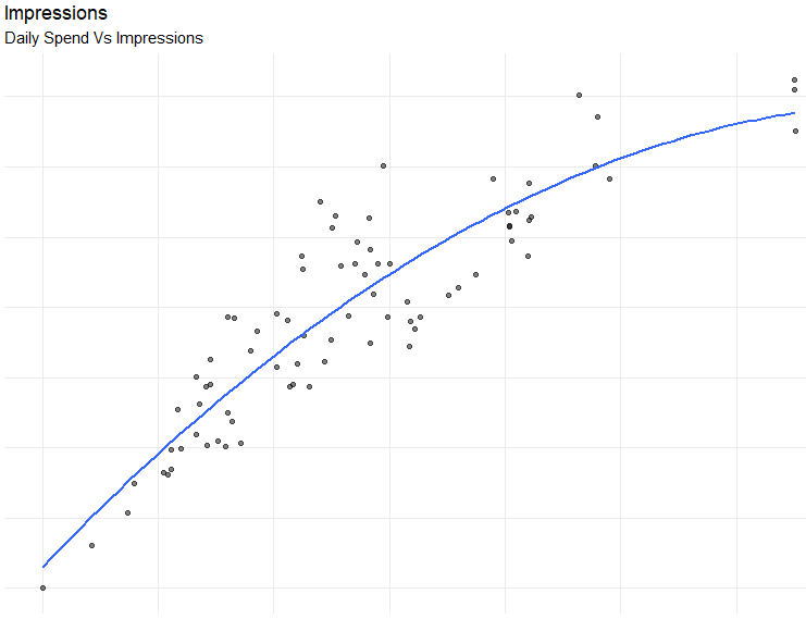
This post discusses how to use polynomial regression for digital advertising data. Polynomial regression can help us better understand the relationship between spend and impressions (or spend and clicks). This method can be particularly useful when looking at daily data with variability in daily spends. Models can be used to analyze, estimate, and benchmark performance of future campaigns. The full code can be found on GitHub.

The code used here uses a second order polynomial function to allow for diminishing marginal returns. For impressions the function takes the form of:

Or in the case of clicks:

To run this code begin by importing the ggplot2, scales, and rio packages.

###############################
## Imports
###############################
imports <- c('ggplot2','scales','rio')
invisible(lapply(imports, require, character.only = TRUE))

First we define a function to fit a second order polynomial regression given two variables. This function also creates a ggplot object that maps a scatter plot of actual observations along with a regression line of predicted values.

FitPolynomial <- function(dat, y, x, d = 2, xlabel = 'x', ylabel = 'y', 
                          title='title', sub.title="x vs. y", caption = "test data"){
  # Perfrom second order polynomial regression of y on x.
  # Args:
  #   dat: data frame containg variables of interest
  #   y: string provding the column name of the dependent variable
  #   x: string providing the column name of the independent variable
  #   d: degree of polynomial to be estimated
  y <- dat[[y]]
  x <- dat[[x]]
  
  poly.fit <- lm(y ~ poly(x, degree = d, raw=TRUE)) # Second order polynomial regression model
  
  plot.out <- ggplot(dat, aes(y=y, x=x)) + # Scatter plot and regression line
    geom_point(alpha = .5) +
    stat_smooth(method="lm", formula = y  ~ poly(x, d, raw = TRUE), se=FALSE)+
    scale_y_continuous(labels = comma) + scale_x_continuous(labels = comma) + theme_minimal() +
    labs(subtitle = sub.title, y = ylabel, x = xlabel, title = title, caption = caption)
  
  list(poly.fit, plot.out)
}

Next we define an objective function. We will pass estimated coefficients from our model to this function and then optimize the function to get a sense for where optimal spend levels may be when assuming diminishing marginal returns.

ObjectiveFunction <- function(B, x){
  # Define second order polynomial as an objective function. This function will be used for optimization.
  # Args: 
  #   B: Vector of estimated coefficients used in second order polynomial regression
  #   x: Integer representing spend level
  B[1] + (B[2]*x) + (B[3]*(x)^2)
}

Similarly we define a function to estimate the predicted values of our dependent variable (impressions or clicks) given a spend level.

EstimateMetric <- function(B, x){
  # Use a second order polynoial function to estimate a metric
  # Args:
  #   B: Vector of estimated coefficients used in second order polynomial regression
  #   x: Integer representing spend level
  round(B[1] + (B[2]*x) + (B[3]*(x)^2))
}

The above code can be edited to fit other functional forms however, in many cases the second order polynomial will suffice.

Finally, we perform regression, estimation, and optimization. The code below uses Impressions and Revenue (Adv Currency) as input data. This is how columns would be named if using daily data from a Google DV360 Report. This method can also be applied to Facebook Ads data and Google Ads data, however the target column names should be changed to reflect the names used in those data sets.

###############################
## Regression, Estimation, and Optimization
###############################
yourdata <- import('path_to_your_data')
y <- 'Impressions'  #name of column containing dependent variable
x <- 'Revenue (Adv Currency)'  #name of column containing independet variable

fit <- FitPolynomial(yourdata, y, x, d = 2) #Fit the model
fit[[2]] #Plot function
#Optimize the objective function given estimated coefficients
fit.optim <- optimize(ObjectiveFunction, B = unname(coef(fit[[1]])), interval = c(100, 10000), maximum = TRUE)
fit.optim
#Estimate value of the objective function at the maximum
EstimateMetric(B = unname(coef(fit[[1]])), x = fit1.optim$maximum)